Introduction to neural networks

Tutorial by Dr. Andrea Santamaria Garcia and Chenran Xu

Get the repository with Git

You will need to have Git previously installed in your computer. To check if you have it installed, open your terminal and type:

git --version

Git installation in mac

brew update
brew install git

Git installation in linux

In Ubuntu/Debian

sudo apt install git

Download the repository

Once you have Git installed open your terminal, go to your desired directory, and type:

git clone https://github.com/machine-learning-tutorial/neural-networks
cd neural-networks

Or get the repository with direct download:

wget https://github.com/machine-learning-tutorial/neural_networks/archive/refs/heads/main.zip
unzip main.zip
cd neural-networks

Install dependencies

You need to install the dependencies before running the notebooks.

Using conda

If you don't have conda installed already and want to use conda for environment management, you can install the miniconda as described here.

Then run the following commands:

conda create -n nn-tutorial python=3.10
conda activate nn-tutorial
pip install -r requirements.txt
jupyter contrib nbextension install --user
jupyter nbextension enable varInspector/main

• After the tutorial you can remove your environment with conda remove -n nn-tutorial --all

Install dependencies

You need to install the dependencies before running the notebooks.

Using venv only

If you do not have conda installed:

Alternatively, you can create the virtual env with venv in the standard library

python -m venv nn-tutorial

and activate the env with $ source /bin/activate (bash) or C:> /Scripts/activate.bat (Windows)

Then, install the packages with pip within the activated environment

python -m pip install -r requirements.txt
jupyter contrib nbextension install --user
jupyter nbextension enable varInspector/main

Running the tutorial

You can start the notebook in the terminal, and it will start a browser automatically

jupyter notebook

Alternatively, you can use supported Editor to run the jupyter notebooks, e.g. with VS Code.

Run this first!

Imports and modules:

%matplotlib inline
import torch
import torch.nn as nn
import h5py
import numpy as np
import matplotlib.pyplot as plt
from IPython.display import set_matplotlib_formats, display
from torch.utils.data import DataLoader, TensorDataset

plt.rcParams['figure.figsize'] = 6, 4
plt.rcParams['savefig.dpi'] = 300
plt.rcParams['image.cmap'] = "viridis"
plt.rcParams['image.interpolation'] = "none"
plt.rcParams['savefig.bbox'] = "tight"

Reproducibility

• We set the random seeds so that the training results are always the same
• Feel free to change the seed number to see the effects of the random initialization of the network weights on the training results

SEED = 26
torch.manual_seed(SEED)
torch.backends.openmp.deterministic = True
np.random.seed(SEED)

Accelerated computing

• Accelerated computing = when we add extra hardware to accelerate computation, like GPUs (needed in deep machine learning).
• GPU: many "not-so-intelligent" cores that are parallelizable. They can carry out specific operations in a very efficient way, e.g. tensor cores perform very efficient sparse tensor multiplication.

We will be working with torch tensors in this notebook! instead of the usual numpy arrays. This means you could execute this code on a GPU if you have access to one with a simple command torch.device("cuda").

# Use GPU if available
device = ('cuda' if torch.cuda.is_available()
          else 'cpu')
print(f'Using {device} device')
# device ='cpu'

Conventions for this notebook

Jargon

• Unit = activation = neuron
• Model = neural network
• Feature = dimension of input vector = number of independent variables
• Hypothesis = prediction = output of the model

Indices

• Data points: $i = 1,..., n$
• Parameters of the model: $k = 1,..., p$
• Layers: $j = 1,..., l$
• Activation unit label: $s$

Scalars

• $u^j$ = number of units in layer $j$
• $z_s^j$ is the activation unit $s$ in layer $j$

Conventions for this notebook

Vectors and matrices

• $\pmb{X}$: input vector of dimension $[n \times (p \times 1)]$
• $z^j$: activation vector of layer $j$ of dimension $[(u^j + 1) \times 1]$
• $\pmb{w}^j$: weight matrix from layer $j$ to $j+1$, of dimension $[u^{j+1} \times (u^j + 1)]$

where the $+1$ accounts for the bias unit

$$ \pmb{X} = \begin{bmatrix} x_0 \\ x_1 \\ \vdots \\ x_p \end{bmatrix} \ \ ; \ \ \pmb{w}^j = \begin{bmatrix} w_{10} & \dots & w_{1(u^j + 1)}\\ w_{20} & \ddots\\ \vdots \\ w_{(u^{j+1}) 0} & & w_{(u^{j+1})(u^j + 1)}\\ \end{bmatrix} $$

Universal Approximation Theorem

• When the activation function is non-linear, then a two-layer neural network can be proven to be a universal function approximator.
• This is where the power of neural networks comes from!

Create a function to fit

Let's create a simple non-linear function to fit with our neural network:

sample_points = 1e3
x_lim = 100
x = np.linspace(0, x_lim, int(sample_points))
y = np.sin(x * x_lim * 1e-4) * np.cos(x * x_lim * 1e-3) * 3
plt.plot(x, y)
plt.xlabel('x')
plt.ylabel('y')
plt.grid()
plt.title('Function to be fitted')

Data shape

• Our data is 1D, meaning it has only one feature.
• We want a model that for a given $x$ it returns the correspondent $y$ value.
• This means that a model with one neuron input and a one neuron output suffices:

n_input = 1
n_out = 1

print(len(x))
print(len(y))

In order for the model to take each point of the data one by one we need to do some additional re-shaping, where we introduce an additional dimension for each entry:

x_reshape = x.reshape((int(len(x) / n_input), n_input))
y_reshape = y.reshape((int(len(y) / n_out), n_out))

# Uncomment to check the shape change
print(x.shape, y.shape)
print(x_reshape.shape, y_reshape.shape)
print(x[10], x_reshape[10])

# print(x_reshape)
# print(x)

PyTorch

PyTorch is an optimized tensor library for deep learning using GPUs and CPUS.

• A tensor is an algebraic object that may map between different objects such as vectors, scalars, and even other tensors. It can be easily understood as a multidimensional matrix/array.
  • These objects allow to easily carry out machine learning computations in problems with many features, weights, etc.
  • In PyTorch, a tensor is a multi-dimensional matrix containing elements of a single data type.

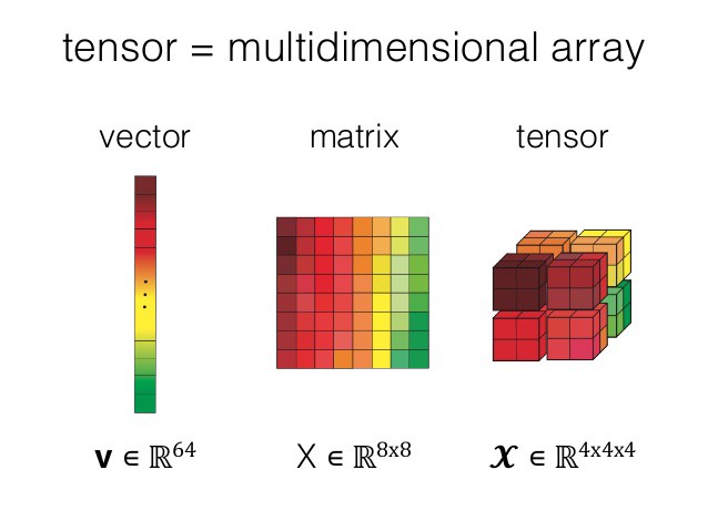
image from Working with PyTorch tensors

Data type

The data that we will input to the model needs to be of the type torch.float32

Side Remark: The default dtype of torch tensors (also the layer parameters) is torch.float32, which is related to the GPU performance optimization. If one wants to use torch.float64/torch.double instead, one can set the tensors to double precision via v = v.double() or set the global precision via torch.set_default_dtype(torch.float64). Just keep in mind, the NN parameters and the input tensors should have the same precision.

Before starting, let's convert our data numpy arrays to torch tensors:

x_torch = torch.from_numpy(x_reshape)
y_torch = torch.from_numpy(y_reshape)

# Type checking:
print(x.dtype, y.dtype)
print(x_torch.dtype, y_torch.dtype)

The type is still not correct, but we can easily convert it:

x_torch = x_torch.to(dtype=torch.float32)
y_torch = y_torch.to(dtype=torch.float32)

# Type checking:
print(x.dtype, y.dtype)
print(x_torch.dtype, y_torch.dtype)

plt.plot(x_torch.numpy(), y_torch.numpy())

Data normalization

We will also need to normalize the data to make sure we are in the non-linear region of the activation functions:

We are using min-max normalization to normalize the input tensors to [0,1] and output tensors to [-0.5,0.5]

x_norm = (x_torch - x_torch.min()) / (x_torch.max() - x_torch.min())
y_norm = (y_torch - y_torch.min()) / (y_torch.max() - y_torch.min()) - 0.5

plt.plot(x_norm.detach().numpy(), y_norm.detach().numpy())
plt.xlabel('x')
plt.ylabel('y')
plt.grid()
plt.title('Normalized function')

x_norm.shape

Build your model

• In PyTorch Sequential stands for sequential container, where modules can be added sequentially and are connected in a cascading way. The output for each module is forwarded sequentially to the next.
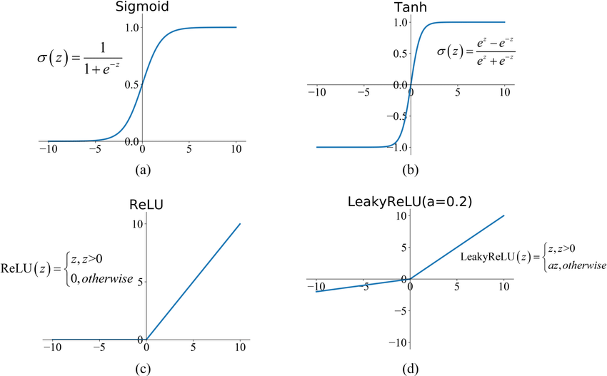
• Now we will build a simple model with one hidden layer with Sequential
• Remember that every layer in a neural network is followed by an activation layer that performs some additional operations on the neurons.

Let's build 3 different models

Model 0

A small model with small non-linearity

n_hidden_01 = 5

model0 = nn.Sequential(nn.Linear(n_input, n_hidden_01),
                      nn.LeakyReLU(),
                      nn.Linear(n_hidden_01, n_out),
                      )
print(model0)

Model 1

A small model with some non-linearity

n_hidden_11 = 5

model1 = nn.Sequential(nn.Linear(n_input, n_hidden_11),
                      nn.Tanh(),
                      nn.Linear(n_hidden_11, n_out),
                      )
print(model1)

Model 2

A larger model with non-linearity

n_hidden_21 = 10
n_hidden_22 = 5
model2 = nn.Sequential(nn.Linear(n_input, n_hidden_21),
                      nn.Tanh(),
                      nn.Linear(n_hidden_21, n_hidden_22),
                      nn.Tanh(),
                      nn.Linear(n_hidden_22, n_out),
                      )
print(model2)

# model2 = nn.Sequential(nn.Linear(n_input, n_hidden_21),
#                       nn.LeakyReLU(),
#                       nn.Linear(n_hidden_21, n_hidden_22),
#                       nn.LeakyReLU(),
#                       nn.Linear(n_hidden_22, n_out),
#                       )
# print(model2)

How much do you think each hyperparameter will affect the quality of the model

$\implies$ uncomment and execute the next line to explore the methods of the model object you created

# dir(model0)

Understanding the PyTorch model

Try the parameters method (needs to be instantiated).

model0.parameters()

The parameters method gives back a generator, which means it needs to be iterated over to give back an output:

for element in model0.parameters():
    print(element)

Without taking into account any bias unit: can you identify the elements of the model by their dimensions?

$\implies$ The first element corresponds to the weight matrix $\theta^0$ from layer 0 to layer 1, of dimensions $u^{j+1} \times u^j = u^2 \times u^1$ (so, without bias)

$\implies$ The second element corresponds to the values of the activation units in layer 1

$\implies$ The third element corresponds to the weight matrix $\theta^1$ from layer 1 to layer 2, of dimensions $u^{j+1} \times u^j = u^3 \times u^3 $ (without bias)

$\implies$ The fourth element is the output of the model

Let's have a look at what the contents of those tensors:

for element in model0.parameters():
    print(element)

What are these values?

Define the loss function

• Reminder: the loss function measures how distant the predictions made by the model are from the actual values
• torch.nn provides many different types of loss functions. One of the most popular ones in the Mean Squared Error (MSE) since it can be applied to a wide variety of cases.
• In general cost functions are chosen depending on desirable properties, such as convexity.

loss_function = nn.MSELoss()

Define the optimizer

torch.optim provides implementations of various optimization algorithms. The optimizer object will hold the current state and will update the parameters of the model based on computer gradients. It takes as an input an iterable containing the model parameters, that we explored before.

learning_rate = 1e-2

optimizer0 = torch.optim.Adam(model0.parameters(), lr=learning_rate)
optimizer1 = torch.optim.Adam(model1.parameters(), lr=learning_rate)
optimizer2 = torch.optim.Adam(model2.parameters(), lr=learning_rate)

# optimizer0 = torch.optim.SGD(model0.parameters(), lr=learning_rate)
# optimizer1 = torch.optim.SGD(model1.parameters(), lr=learning_rate)
# optimizer2 = torch.optim.SGD(model2.parameters(), lr=learning_rate)

Train the models on a loop

The model learns iteratively in a loop of a given number of epochs. Each loop consists of:

• A forward propagation: compute $y$ given the input $x$ and current weights and calculate the loss
• A backward propagation: compute the gradient of the loss function (error of the loss at each unit)
• Gradient descent: update model weights

batch_size = 64 # how many points to pass to the model at a time
# batch_size = len(x_norm)  # uncomment to pass all data at once
dataset = TensorDataset(x_norm, y_norm)
dataloader = DataLoader(dataset, batch_size=batch_size, shuffle=True, pin_memory=False, drop_last=True)

# Define the training loop NEW
def training_loop(dataloader, model, optimizer, epochs):
    losses = []
    for _ in range(epochs):
        for id_batch, (x_batch, y_batch) in enumerate(dataloader):
            x_batch = x_batch.to(device)
            y_batch = y_batch.to(device)
            pred_y = model(x_batch)
            optimizer.zero_grad()
            loss = loss_function(pred_y, y_batch)
            loss.backward()  # Back-prop
            optimizer.step()
            losses.append(loss.item())
    return losses

# Run the training for all the models
# epochs = 2000
epochs = 500

losses0 = training_loop(dataloader, model0, optimizer0, epochs=epochs)
losses1 = training_loop(dataloader, model1, optimizer1, epochs=epochs)
losses2 = training_loop(dataloader, model2, optimizer2, epochs=epochs)

plt.plot(losses0, label='Model 0', color='green')
plt.plot(losses1, label='Model 1', color='blue')
plt.plot(losses2, label='Model 2', color='red')
plt.ylabel('Loss')
plt.xlabel('Epoch')
plt.title("Learning rate %f"%(learning_rate))
plt.legend()
plt.show()

Interpreting the loss curves

$\implies$ Have the NNs learned?

$\implies$ Why is model 0 learning faster than model 1?

$\implies$ Why is model 2 better than models 0 and 1?

$\implies$ Train for more epochs. How does the loss curve change?

$\implies$ Change the number of minibatches to pass all data at once. How does the loss curve change? which method is more effective

Test the trained model

• Let's create some random points in the x-axis within the model's interval that will serve as test data.
• We will do the same data manipulations as before.

test_points = 50
x_test = np.random.uniform(0, np.max(x_norm.detach().numpy()), test_points)
x_test_reshape = x_test.reshape((int(len(x_test) / n_input), n_input))
x_test_torch = torch.from_numpy(x_test_reshape)
x_test_torch = x_test_torch.to(dtype=torch.float32)

Now we predict the y-value with our model:

y0_test_torch = model0(x_test_torch)
y1_test_torch = model1(x_test_torch)
y2_test_torch = model2(x_test_torch)

plt.plot(x_norm.detach().numpy(), y_norm.detach().numpy())
plt.scatter(x_test_torch.detach().numpy(), y0_test_torch.detach().numpy(), color='green', marker='*', label='Model 0')
plt.scatter(x_test_torch.detach().numpy(), y1_test_torch.detach().numpy(), color='blue', marker='v', label='Model 1')
plt.scatter(x_test_torch.detach().numpy(), y2_test_torch.detach().numpy(), color='red', label='Model 2')
plt.legend()
plt.show()

Comment on the NN predictions

$\implies$ Why does the prediction of model 0 have that particular shape?

$\implies$ Which activation function would be more appropriate to fit this function, the one from model 0 or model 1?

$\implies$ Which NN gets the best prediction and why?

Bonus

$\implies$ Change the seed at the top of the notebook. How do the predictions change?

$\implies$ Change the optimizer in Section 4 from Adam to SGD and re-train the models. What happens? How did the loss curves change? Did the NNs learn? Change the number of epochs and try to make it learn.

Play with the notebook!

Some ideas:

• Change the number of epochs in Section 5 to 5000 and re-train the models. What happens?
• Change the random seed in the Reproducibility cell at the very top. How do the results change?
• Change the optimizer in Section 4 from Adam to SGD and re-train the models. What happens?
• [if time allows, takes several minutes] Change the epochs in Section 5 to 1000000. What happens?
• Go back to 1000 epochs and the Adam optimizer. Change the learning rate in Section 4 to 0.05. How do the results change? what does it tell us about our previous value?
• Change the learning rate to 0.5. What happens now?